
Research | Open Access | Volume 9 (Suppl 12): Article 15 | Published: 28 Aug 2026

Views: 3,124
Menu, Tables and Figures
| Parameter | Description | Values-1 | Units | Reference |
|---|---|---|---|---|
| λₕ | Recruitment rate of humans | 0.34 | week⁻¹ | Estimated |
| βₕᵣ | Transmission rate from rodents to humans | 0.0509 | week⁻¹ | Fitted |
| βₕₕ | Transmission rate from humans to humans | 0.196 | week⁻¹ | Fitted |
| βₑᵥ | Transmission rate from environment to humans | 0.028 | week⁻¹ | Fitted |
| μₕ | Natural death rate of humans | 0.00133 | week⁻¹ | Estimated |
| P | Proportion of asymptomatic infections | 0.8 | dimensionless | [13] |
| σₕ | Progression rate from exposed to infectious | 0.16136 | week⁻¹ | Fitted |
| γₕ | Recovery rate of humans | 0.1122 | week⁻¹ | Fitted |
| δₕ | Disease-induced death rate in humans | 0.0189 | week⁻¹ | [9] |
| ωₕ | Rate of immunity loss in humans | 0.03278 | week⁻¹ | [4] |
| λᵣ | Recruitment rate of rodents | 0.05 | week⁻¹ | [27] |
| βᵣᵣ | Transmission rate among rodents | 0.0254 | week⁻¹ | [17][27] |
| μᵣ | Natural death rate of rodents | 0.0192 | week⁻¹ | Estimated |
| σᵣ | Progression rate in rodents | 0.004 | week⁻¹ | [4] |
| Η | Contamination rate by infected rodents | 0.046 | week⁻¹ | Estimated |
| Ξ | Clearance rate of the environment | 0.078 | week⁻¹ | [28] |
Table 1: Parameters used in the model and their description
| Parameter | Description | Sensitivity Index | Interpretation |
|---|---|---|---|
| βhh | Human-to-human transmission rate | + 1.00 | A 1% increase in βhh increases R0 by 1% (strongest positive driver) |
| γh | Human recovery rate | – 0.73 | A 1% increase in γh decreases R0 by 0.73% (strongest negative driver) |
| δh | Disease-induced death rate | – 0.246 | A 1% increase in δh decreases R0 by 0.246% |
| σh | Progression rate (exposed → infectious) | + 0.0207 | Negligible positive effect |
| μh | Natural death rate of humans | – 0.04 | Negligible negative effect |
Table 2: Normalized forward sensitivity indices of R_0 to key parameters.
Polycarp Dauda Madaki1, Olalekan Taiwo2, Oghenetega ThankGod Oweh3,&, Sylvia Adanma Ezenwa-Ahanene4, Zubairu Dalhatu Zubairu5, Charles Obi2, Ganiyat Eshikhena2, Dupsy Akoma2, Ezra Gayawan6, Ruth Manzo Sabo7, Zainab Dambazau4, Jide Idris4, Oladipo Ogunbode4, Chijioke Kaduru2
1Department of Veterinary Tropical Diseases, University of Pretoria, Pretoria 0110, South Africa, 2Corona Management System, Abuja, Nigeria, 3Department of Medical Biochemistry, College of Medicine, Kaduna State University, 4Nigeria Centre for Disease Control and Prevention (NCDC), 5Department of Public Health, Faculty of Basic and Applied Biological Sciences, Ahmadu Bello University, DLC, Zaria, Nigeria, 6Department of Statistics, Federal University of Technology, Akure, Nigeria, 7African Centre for Disease Control and Prevention, Addis Ababa, Ethiopia
&Corresponding author: Oghenetega ThankGod Oweh, Department of Medical Biochemistry, College of Medicine, Kaduna State University, Email: oghenetega.oweh@kasu.edu.ng ORCID: https://orcid.org/0000-0002-0051-9975
Received: 13 Dec 2025, Accepted: 18 Aug 2026, Published: 28 Aug 2026
Domain: Infectious Disease Epidemiology, Disease Modelling
Keywords: Lassa Fever, SEIR-SEI model, Spatial, Rodent, One Health
©Polycarp Dauda Madaki et al. Journal of Interventional Epidemiology and Public Health (ISSN: 2664-2824). This is an Open Access article distributed under the terms of the Creative Commons Attribution International 4.0 License (https://creativecommons.org/licenses/by/4.0/), which permits unrestricted use, distribution, and reproduction in any medium, provided the original work is properly cited.
Cite this article: Polycarp Dauda Madaki et al. Spatiotemporal and compartmental modelling of Lassa fever transmission dynamics in Nigeria. Journal of Interventional Epidemiology and Public Health. 2026; 9(Suppl 12):15. https://doi.org/10.37432/jieph-d-25-00322
Introduction: Lassa fever (LF) is a zoonotic haemorrhagic fever endemic to West Africa, with 300,000-500,000 annual cases. In Nigeria, transmission dynamics are poorly understood due to limited integration of ecological, spatial, and temporal drivers.
Methods: We combined spatiotemporal and compartmental modelling using confirmed LF incidence data from the Nigeria Centre for Disease Control (NCDC, 2018-2024). A deterministic SEIAR (Susceptible-Exposed-Asymptomatic-Symptomatic-Recovered) model for humans coupled with an SEI model for rodents and an environmental contamination compartment was formulated (16 parameters). The Next-Generation Matrix (NGM) yielded the basic reproduction number (R_0 ). Global Moran’s I and Local Indicators of Spatial Association (LISA) identified hotspots. Time series decomposition and ARIMA modelling forecasted 2025–2028 incidence. Scenario analyses compared rodent control versus healthcare improvement.
Results: NGM estimated R_0=1.66, higher than empirical estimates (≈1.0), indicating underappreciated zoonotic transmission. Sensitivity analysis identified human-to-human transmission rate (β_hh=+1.0) as the most positive driver and recovery rate (γ_h=- 0.73) as the most negative. Rodent population reduction (70%) reduced infections by 61.7%, compared to a 16.1% reduction from equivalent healthcare improvement. This represents a 3.8-fold greater efficacy of reservoir-targeted interventions. Spatial analysis revealed significant clustering (Global Moran’s I = 0.138, p = 0.027) with persistent hotspots in Edo and Ondo states (p < 0.01). Temporal analysis confirmed seasonality (ARIMA residuals, p = 0.381) and forecasted peak incidence of ≈350 cases in 2025–2028.
Conclusion: Integrated One Health strategies prioritising rodent control alongside healthcare strengthening are most effective. Our spatial-temporal-compartmental framework provides actionable evidence for targeted LF control in Nigeria.
Lassa virus (LASV) is a zoonotic, acute, and fatal viral haemorrhagic fever that is found in parts of West Africa, including Sierra Leone, Liberia, Guinea and Nigeria [1]. It is spread by the “multimammate rat” ( Mastomys natalensis), which is found throughout Sub-Saharan Africa [2]. Lassa fever virus (LASV), a member of the family Arenavirus, is a significant cause of morbidity and mortality: annually, 300,000–500,000 infection cases, resulting in 5000 deaths [3]. While Lassa fever is mild or has no observable symptoms in about 80% of people infected with the virus, the remaining 20% suffer from a severe disease [4]. Ramzan et al [5] showed the relationship between Lassa fever and several disabilities, including encephalitis, hearing loss, ataxia, neuropsychiatric manifestations, meningitis, seizures, and coma.
The incubation period of Lassa fever (LF) is between 6 and 21 days, after which infected individuals may start showing symptoms ranging from mild to severe, including neurological complications and respiratory failure [6]. Lassa fever accounts for 6.0% of fevers, 0.7% of hospital admissions, 40% of the case fatality rate (CFR), and almost a quarter of maternal mortality during its peak in West Africa [7]. Lassa Fever affects all age groups in endemic regions, especially impoverished rural communities [8].
Lassa fever incidence in Nigeria has reached an alarming new stage. Surveillance data show a rising number of cases in non-endemic states from 2015 to 2024 [9], coinciding with rodent habitat expansion due to deforestation and urban growth [10]. The geographic spread of the epidemic worsens existing challenges in Nigeria since less than thirty per cent of states have reliable polymerase chain reaction (PCR) testing capacity [11], which might lead to substantial underreporting of Lassa fever cases.
The direct and indirect expenses from Lassa fever outbreaks present a high financial burden for Nigeria [12]. The healthcare sector assumes most expenses related to these occurrences by spending heavily on disease management, outbreak response and preventive measures [8].
Lassa fever exhibits marked seasonality. Although outbreaks can occur at any time of year, transmission peaks during the dry season due to increased human-rodent interactions [13]. Knowledge of the spatial and temporal dynamics of Lassa fever to inform effective public health interventions and policies has been highlighted by prior studies [7, 13]. A study that analysed national surveillance data and observed a recent increase in both the number and geographic spread of Lassa fever cases in Nigeria highlighted the need for specific targeted control measures [7].
Similarly, a study by McKendrick et al [13] developed a mathematical model incorporating rodent population dynamics to highlight the seasonal peaks in human cases, emphasizing the role of environmental factors in disease transmission. Ramzan et al [14] reported, from a sensitivity analysis study, the importance of holistic control that leverages medical treatment with rodent population control and improved environmental hygiene. Fractional-order modelling has been successfully applied to various infectious diseases, including chlamydia with protected intimacy as a strategic control intervention [15], malaria and measles co-infections with public awareness interventions [16], and Lassa fever with non-pharmaceutical interventions under optimal control [17], demonstrating the broader applicability of memory-dependent epidemic models across different disease systems.
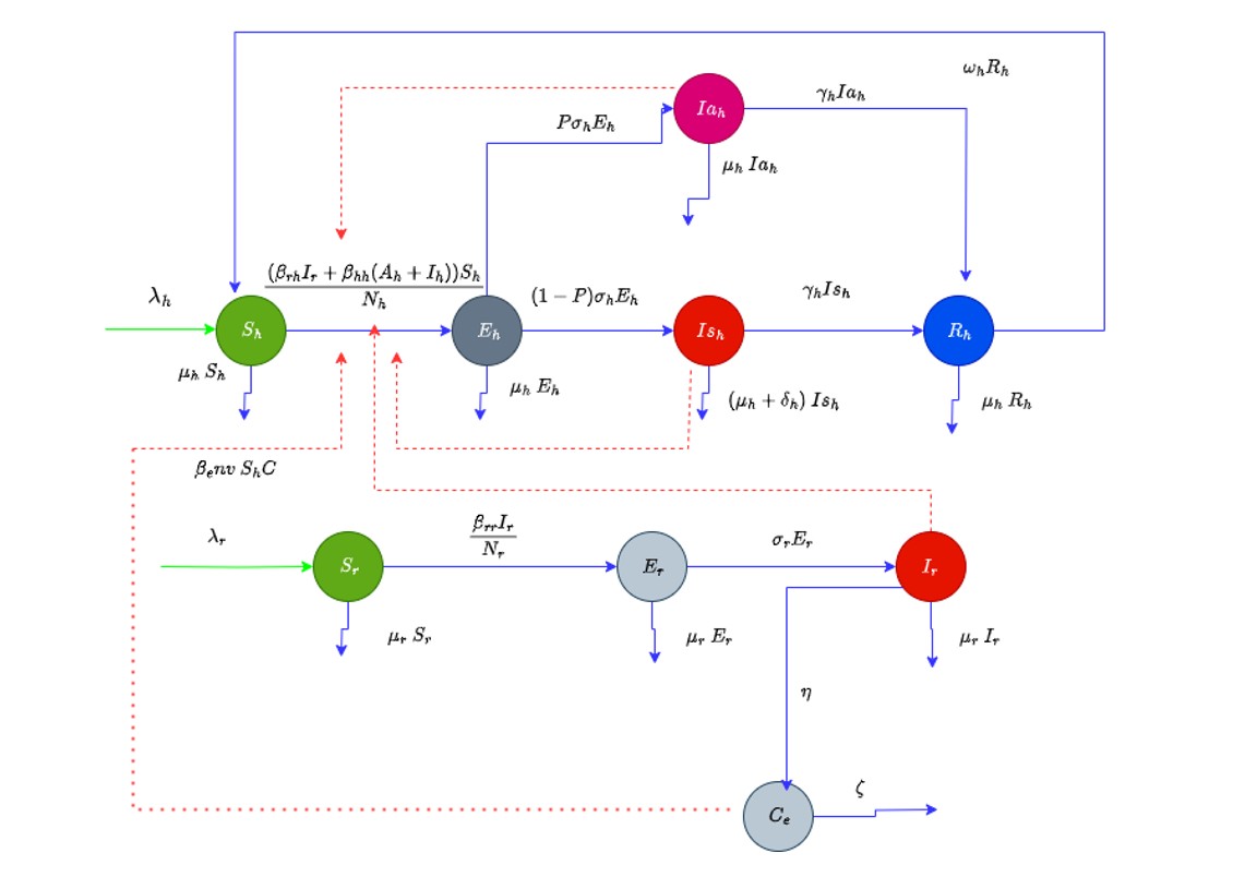
Lassa fever remains a significant national health threat in Nigeria, as outbreaks have persisted and there has been a high level of spatial disparity in the distribution of the disease. This study aims to integrate spatiotemporal and compartmental modelling approaches to characterize Lassa fever transmission dynamics in Nigeria and evaluate control strategies Specifically, this study aims to: estimate the basic reproduction number (R_0 ) using three methods (attack rate, incidence data, and next-generation matrix); identify spatial hotspots and temporal seasonality; quantify the impact of rodent control versus healthcare interventions through scenario analysis; and forecast future incidence (2025–2028). Figure 1 illustrates the multi-host, multi-route transmission framework underpinning our modelling approach. Figure 1 (schematic diagram of transmission pathways) illustrates the multi-host, multi-route transmission framework between humans, rodent reservoirs, and environmental contamination, which underpins our modelling approach.
This study combines three contributions that aid the understanding of Lassa fever transmission in Nigeria. Unlike prior Lassa fever models that focus solely on compartmental dynamics or spatiotemporal patterns in isolation, this study integrates a multi-host SEIAR-SEI model with environmental contamination, geospatial hotspot analysis (Global Moran’s I, LISA), and time series forecasting (ARIMA) within a single framework. Furthermore, the study directly compares three R_0 estimation methods (attack rate, incidence, next-generation matrix) to reveal a critical discrepancy between empirical and mechanistic transmission potential. This study also quantified the differential efficacy of rodent control versus healthcare improvement at equivalent implementation levels, providing evidence-based priorities for One Health interventions in Nigeria.
Study design and data source
This is a mathematical modelling study based on secondary surveillance data. Epidemiological data on Lassa fever confirmed cases (weekly incidence, 2018-2024) were obtained from the Nigeria Centre for Disease Control (NCDC) via the Integrated Disease Surveillance and Response system (IDSR). Cases were laboratory-confirmed by PCR at reference laboratories [9]. Demographic and environmental data (population density, housing conditions, healthcare facility access) were sourced from the Multiple Indicator Cluster Survey (MICS) conducted by the National Bureau of Statistics (NBS) with UNICEF support [18]. The temporal unit of analysis was weekly confirmed cases aggregated at the state level. A confirmed case was defined according to NCDC guidelines: a person with fever (≥38.0°C) or a history of fever in the past 21 days, not responding to antimalarials or antibiotics, with at least one of the following: sore throat, myalgia, chest pain, nausea/vomiting, diarrhoea, cough, or abdominal pain, and laboratory confirmation via reverse-transcription polymerase chain reaction (RT-PCR) at an NCDC reference laboratory [9].
Model formulation
We extended an SEIAR (humans) and SEI (rodents) framework incorporating environmental contamination. The human population is divided into five compartments: susceptible (S_h), exposed (E_h), asymptomatic infected (I_Ah), symptomatic infected (I_Sh), and recovered (R_h). The rodent population has three compartments: susceptible (S_r), exposed (E_r), and infected (I_r). The environment (C) represents viral contamination from infected rodents.
The total populations for humans and rodents at any time (t) are defined as:
$$\begin{align}
N_h(t) &= S_h(t) + E_h(t) + I_{Ah}(t) + I_{Sh}(t) + R_h(t) \tag{1} \\
N_r(t) &= S_r(t) + E_r(t) + I_r(t) \tag{2}
\end{align}$$
The model combines numerous crucial parameters that guides the transmission dynamics of Lassa fever. For the human population, λ_h denotes human recruitment rate by birth or immigration. Susceptible humans (S_h ) can become exposed through contact with infected rodents at a transmission rate β_rh, through contact with infected humans at a transmission rate β_hh, or by environmental contamination at a rate β_env. Natural mortality occurs at a rate μ_h. Exposed individuals 〖(E〗_h) progress to the infectious class at a rate σ_h, with a proportion (P) becoming asymptomatic infected I_Ah and the remaining (1-P) becoming symptomatic infected (I_sh). Infected individuals recover at a rate γ_h, while symptomatic infections may result in disease-induced mortality at a rate δ_h. Recovered individuals (R_h ) lose immunity at a rate ω_h, re-entering the susceptible population.
For the rodent population, λ_r denotes the recruitment rate through birth, while S_r represents susceptible rodents that become exposed through contact with infectious rodents at a transmission rate β_rr, Exposed rodents (E_r ) progress to the infectious class I_r at a rate σ_r. Natural mortality affects both susceptible and infectious rodents at a rate μ_r. The environmental compartment(C), signifies contamination from infectious rodents, with a rate η. Rate ξ represents clearance of the contaminated environment.
Model assumptions
There are six important assumptions that underline the model. First, homogeneous mixing is assumed within human and rodent populations, which simplifies transmission dynamics but may overestimate spread in spatially heterogeneous settings; this can be relaxed in future agent-based or metapopulation models. Second, the rodent to human ratio is set as 1:1, but the ratio fluctuates seasonally and according to land use and can be expanded to include dynamic rodent birth rates as a function of climate variables in future research. Third, recovery does not provide permanent immunity ω_h>0 , as there is evidence of declining antibody levels in Lassa survivors over time. Fourth, environmental contamination is modelled as a single compartment C in which the decay is linear, and spatial heterogeneity in viral persistence is not accounted for; a partial differential equation model could relax this. Fifth, changes in human behaviour during outbreaks (e.g. reduced contact) are not accounted for, which could overestimate peak incidence; adaptive transmission rates can be used to incorporate behavioural feedback. Sixth, these parameter values were selected from literature (when available), by using a demographic estimation and/or by fitting them to the NCDC data, as explained in the Parameter Estimation section. Parameters that were highly sensitive β_hh,γ_h were selected for accurate fitting
Model equations
The Lassa fever model in Figure 1 is expressed as a system of first-order nonlinear ordinary differential equations as follows:
$$\begin{align}
\frac{dS_r}{dt} &= \lambda_r – \frac{\beta_{rr} I_r}{N_r} S_r – \mu_r S_r \tag{8} \\[10pt]
\frac{dE_r}{dt} &= \frac{\beta_{rr} I_r}{N_r} S_r – (\sigma_r + \mu_r) E_r \tag{9} \\[10pt]
\frac{dI_r}{dt} &= \sigma_r E_r – \mu_r I_r \tag{10}
\end{align}$$
$$\begin{align}
\frac{dC}{dt} &= \eta I_r – \xi C \tag{11}
\end{align}$$
The total progression rate out of the exposed human compartment is \(\sigma_h\), with fraction \(P\) entering \(I_{ah}\) (asymptomatic) and fraction \((1-P)\) entering \(I_{sh}\) (symptomatic). This ensures conservation of population flow: \(\frac{dE_h}{dt}\) losses = \((\sigma_h + \mu_h)E_h\)
Basic properties of the model
Invariant region
The invariant region is the set of all possible states of the system where the solutions remain non-negative and bounded. We assume the total human population N_h and the total rodent population N_r are constant.
Total human population:
The derivative of \(N_h\) is:
Substituting the equations:
At equilibrium \(\frac{dN_h}{dt} = 0\)
Total rodent population:
The derivative of \(N_r\)
Substituting the equations
At equilibrium \(\frac{dN_r}{dt} = 0\):
Positivity of solutions
To ensure the solutions remain non-negative for all time, we check the derivatives when each compartment is zero.
Susceptible humans (\(S_h\))
This is non-negative since \(\lambda_h > 0\) and \(\omega_h R_h \geq 0\)
Exposed humans (\(E_h\))
This is non-negative since all terms are \(\geq 0\)
Asymptomatic infected humans (\(I_{Ah}\))
This is non-negative since \(P \sigma_h E_h \geq 0\)
Symptomatic infected humans (\(I_{Sh}\))
This is non-negative since \((1 – P) \sigma_h E_h \geq 0\)
Susceptible rodents (\(S_r\))
This is non-negative since \(\lambda_r \geq 0\)
Exposed rodents (\(E_r\))
This is non-negative since all terms are \(\geq 0\)
Infected rodents (\(I_r\))
This is non-negative since \(\sigma_r E_r \geq 0\)
Contaminated environment (\(C\))
This is non-negative since \(\eta I_r \geq 0\)
Recovered humans (\(R_h\))
This is non-negative since \(\gamma_h (I_{Ah} + I_{Sh}) \geq 0\)
Boundedness of solutions
We have already shown that the total populations \(N_h\) and \(N_r\) are bounded. Since all compartments are subsets of \(N_h\) and \(N_r\), they are also bounded.
Human population
Rodent population:
Thus, every solution of the model with initial condition in \(\Omega\) remains there for \(t > 0\). It follows that \(\Omega\) is positive invariant. Hence it is sufficient to consider the dynamics of the flow generated by the equations in \(\Omega\). In this region, the model can be considered as being epidemiologically and mathematically well-posed.
Scaling of the model
To simplify the analysis of the Lassa fever model equation, the population ratios are determined by scaling each class relative to the total population of the species to get the initial states. Given different populations N(t),the proportion of each category within the population is expressed as:
Following previous modelling studies [14], we assumed a 1:1 ratio of rodents to humans in Nigeria, giving an initial rodent population \(N_r(0) = N_h(0) \approx 2.2 \times 10^8\). Therefore \(S_h = s_H N_h\), \(E_h = e_H N_h\), \(I_{Ah} = i_{AH} N_h\), \(I_{Sh} = i_{SH} N_h\), \(R_h = r_H N_h\), and \(S_r = s_R N_r\), \(E_r = e_R N_r\), \(I_r = i_R N_r\).
Parameter estimation
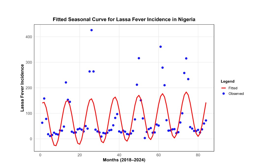
Table 1 outlines the parameter estimation strategies employed for our SEIR-SEI model, which includes a total of sixteen parameters. Of these, realistic values for seven were sourced directly from existing literature. Four demographic parameters, the recruitment rates and natural death rates for both humans and rodents, as well as the environmental contamination rate caused by infected rodents, were estimated. Other parameters such as rodent-to-human transmission rates, human-to-human transmission rates, environment to rates, progression rate from exposed to infectious and human recovery rate were determined by fitting the model to the Lassa fever case data (Figure 2) collected between 2018 and 2024 from the Nigeria Centre for Disease Control (NCDC). Parameters marked ‘fitted’ \(\beta_{rh}, \beta_{hh}, \beta_{env}, \sigma_h, \gamma_h\) were estimated by fitting the model to weekly confirmed Lassa fever incidence data from NCDC (2018-2024) using nonlinear least squares in R (v4.3.1) with the nls function. Initial guesses were derived from literature values for related zoonotic diseases. Parameters marked ‘estimated’ \(\lambda_h, \mu_h, \mu_r, \eta\) were calculated from demographic data: \(\lambda_h\) from Nigeria’s crude birth rate, \(\mu_h\) from life expectancy, \(\mu_r\) from rodent life expectancy (\(\approx 1\) year), and \(\eta\) was calibrated to match environmental persistence reported in the literature. The sinusoidal function used was \(I_{pred}(t) = a + b t + c \sin(2\pi t / 52 + \phi)\), where \(t\) is in weeks.
Numerical simulation
The system of ordinary differential equations (ODEs) (Equations 3-11) was solved numerically using the fourth-order Runge-Kutta (RK4) method with a fixed time step of Δt = 0.01 weeks (approximately 1.68 hours). The RK4 scheme was chosen for its balance of accuracy and computational efficiency for non-stiff deterministic ODE systems. The time step was selected to be sufficiently smaller than the fastest process rate (ξ = 0.078 week⁻¹) to ensure numerical stability. Model implementation and parameter fitting were performed in R version 4.3.1 using the deSolve package
Basic reproduction number (\(R_0\))
The basic reproduction number of an infectious disease is defined as the average number of secondary cases emanating from one infected individual in a population totally susceptible to infection. To estimate the basic reproduction number (\(R_0\)) for Lassa fever in Nigeria, three different methods were employed based on both estimated parameters and parameters from the literature, which include attack rate (AR), incidence data, and the Next Generation Matrix (NGM) approach.
The DFE is:
The model equations (4)–(6) and (9)–(10) are rewritten as \(\frac{dx}{dt} = F(x) – V(x)\),
where F represents new infections and V represents all other transfers (progression, mortality, recovery). The Jacobian matrices of F and V evaluated at the DFE are partitioned as:
The nonzero entries of F (new infections) are:
The V matrix (transfers out) is diagonal for progression and mortality:
The inverse \(V^{-1}\) is computed analytically. The next-generation matrix is \(K = F V^{-1}\). The basic reproduction number \(R_0\) is the spectral radius (largest eigenvalue) of K:
Where:
And
Since we model spillover from rodents to humans, the overall \(R_0\) for the human epidemic is dominated by human-to-human transmission
The vectors of new infections \(F\) and other transfers \(V\) are derived from Equations (4)–(6) and (9)–(10). The Jacobian matrices at the DFE are partitioned. The \(F\) matrix (new infections) has non-zero entries corresponding to transmission pathways:
The \(V\) matrix (transfers out of compartments) is diagonal for progression and mortality terms. The inverse \(V^{-1}\) is computed analytically. The product \(F V^{-1}\) is a \(5 \times 5\) matrix. Its spectral radius \(\rho(F V^{-1})\) yields the largest eigenvalue, which simplifies to:
Where:
and
Since we are modelling spillover from rodents to humans, the overall \(R_0\) for the human epidemic is driven by the human-to-human transmission chain, yielding Equation (37)
Stationarity analysis and time series decomposition
Stationarity of the time series was tested using the Augmented Dickey-Fuller (ADF) test. The test was conducted with a lag order of 4 to account for autocorrelation, and the alternative hypothesis was set to stationary. The data on the occurrence of Lassa fever (2018–2024) was subjected to time-series analysis to determine the trends, seasonality, and predict future trends. Classical decomposition was initially used to decompose the series into trend, seasonal and random. The Augmented Dickey-Fuller (ADF) test was used to test stationarity. The Box-Jenkins approach was adopted, after which an ARIMA model with seasonal adjustments was fitted to the data. The Autocorrelation Function (ACF) and Partial Autocorrelation Function (PACF) plots were used to identify lag orders of autoregressive (AR), moving average (MA) and seasonal terms, and the best-fitting model was chosen based on the lowest Akaike Information Criterion (AIC) and Bayesian Information Criterion (BIC) values. Box-Ljung test and residual diagnostics were used to assess model adequacy and independence, and the behaviour of white noise. The validated model was then applied to come up with forecasts of Lassa fever incidence in 2025-2028 with 95% prediction intervals.
Geospatial mapping
The 2018 to 2024 data on the prevalence of Lassa fever in Nigeria were analyzed using geospatial analysis to provide an opportunity to study the spatial and temporal distribution of the cases. The prevalence was put on a 100,000-population basis so that it could be compared across states. Global Moran’s I was used to determine the degree of spatial autocorrelation to confirm the existence of general clustering, whereas Local Moran I (LISA) was used to establish the presence of meaningful hotspots and cold spots at the state level. Annual variations in the clustering were analyzed through annual Moran I with Queen contiguity spatial weights. To examine the possible determinants of Lassa fever, Ordinary Least Squares (OLS) regression was used, in which cumulative prevalence was the dependent variable and the independent variables included population size, primary healthcare coverage, total healthcare access, and environmental indicators (housing conditions). R2, adjusted R2, predictor significance and Moran’s I test with residuals were used to indicate model diagnostics and measure residual spatial autocorrelation.
Numerical simulations
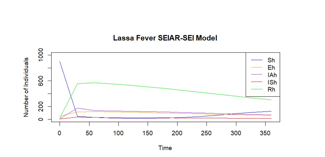
The numerical parameters in Table 1 and the initial states S_h (0)= 0.81, E_h (0)=0.08, I_Ah (0)=0.056, I_sh (0)=0.014, R_h (0)=0.04 and S_r (0)=0.83, Er(0)=0.09, Ir(0)=0.08 were used. Time series plots of the model with different initial conditions are presented in Figure 3.
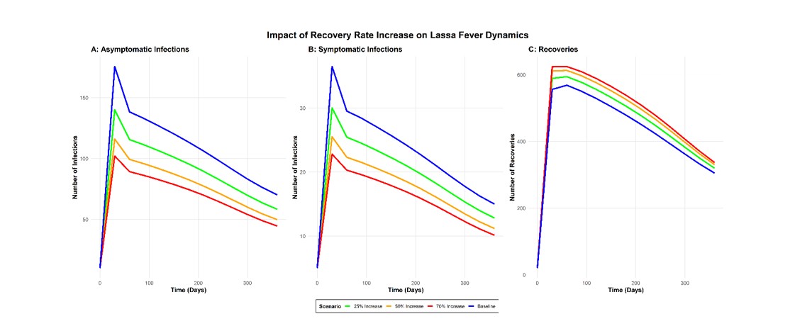
The scenario analysis as indicated in Figure 4 shows how changes in the recovery rate affect both infections and recoveries over the course of the simulation. The results for infection change indicate that as the recovery rate increases, the total number of symptomatic and asymptomatic infections decreases. Specifically, when the recovery rate is increased by 25%, the infections reduce by around 16.07%. When the recovery rate is increased by 50%, the infections decline by approximately 27.63%, and when the recovery rate is increased by 70%, the infections reduce by 34.77%. This shows that an increase in the recovery rate can cause a reduction in the burden of infections quite significantly, as individuals recover sooner, and thus fewer individuals become infected, and disease transmission is decreased.
Similarly, a change in the recovery rate has an impact on the overall recovery number. If the recovery rate goes up by 25%, the recoveries go up by 5.36%. When increased by 50%, recoveries go up by 9.27%, and when increased by 70%, recoveries go up by 11.72%. These results demonstrate a positive relationship between the recovery rate and the number of recoveries, indicating that faster recovery contributes to a larger proportion of the population recovering over time.
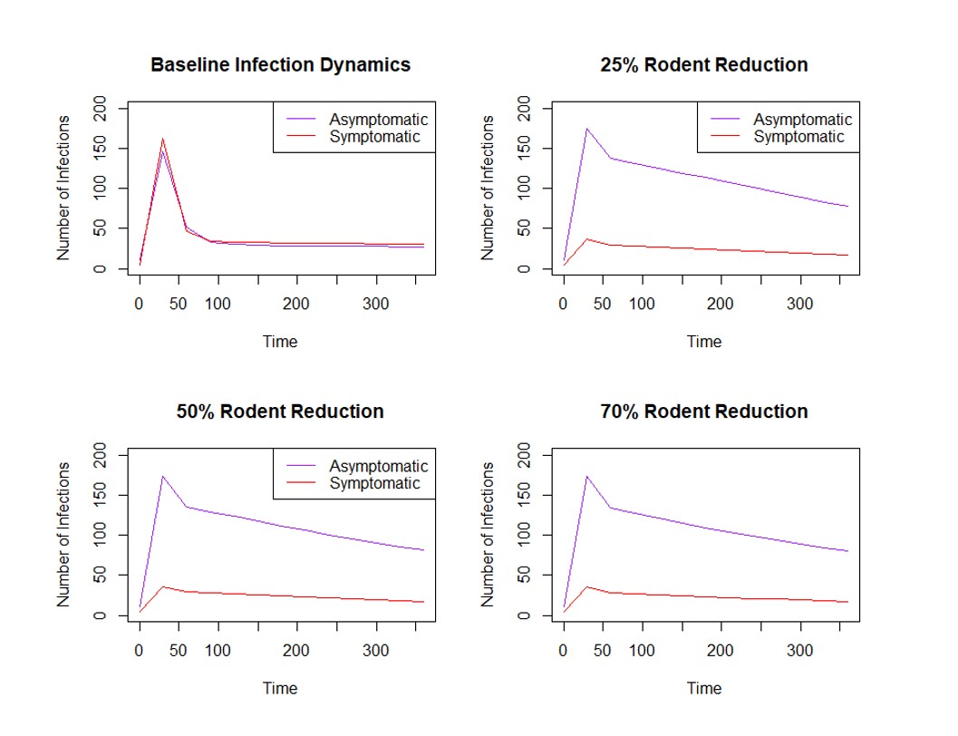
The scenario analysis of rodent population reduction, as shown in Figure 5, displays the impact of rodent control on the infection rate of Lassa fever. Decreasing the rodent population by 25% resulted in a reduction in infections by 58.47%. Decreasing the rodent population by 50% resulted in the infection rate going down by 61.05%. Lowering the rodent population further by 70% resulted in infections going down by 61.7%.
Sensitivity analysis
The normalised forward sensitivity index \(Z_p^{R_0}\) the reproduction number \(R_0\) for each of the parameters is defined as
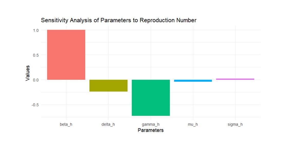
The sensitivity analysis as shown in Figure 6 reveals that the transmission rate (\(\beta_h\)) has a strong positive effect on the reproduction number, with a value of 1. Conversely, both the death rate due to Lassa fever (\(\delta_h\)) and the recovery rate (\(\gamma_h\)) exhibit negative effects, with values of -0.246 and -0.73, respectively. The natural death rate (\(\mu_h\))and the disease progression rate (\(\sigma_h\)) show minimal impact, registering at -0.04 and 0.0207, respectively. The normalized forward sensitivity indices (Table 2) quantify the elasticity of \(R_0\) to each parameter. The human-to-human transmission rate (\(\beta_{hh} = +1.00\)) is the most positive driver: a 1% increase in \(\beta_{hh}\) increases \(R_0\) by 1%. Conversely, the human recovery rate (\(\gamma_h = -0.73\)) is the strongest negative driver: a 1% increase in \(\gamma_h\) reduces \(R_0\) by 0.73%. The disease-induced death rate ((\(\delta_h = -0.246\)) has a moderate negative effect, while natural death (\(\mu_h = -0.04\)) and progression rate (\(\sigma_h = +0.0207\)) have negligible impacts. These indices identify \(\beta_{hh}\)and \(\gamma_h\)as the most influential targets for intervention.
Basic reproduction number (\(R_0\))
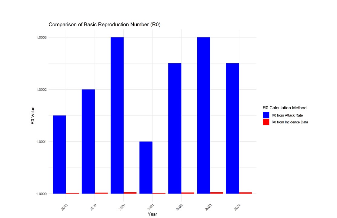
Analysis of \(R_0\) from 2018 to 2024, as shown in Figure 7 reveals a remarkably stable transmission dynamic. From 2018 to 2024, \(R_0\) estimates derived from both attack rates and incidence data remained consistently close to 1, with minimal fluctuations. Attack rate-derived \(R_0\) ranged from 1.00010 to 1.00030, while incidence-derived \(R_0\) ranged from 1.000001 to 1.000003. While the attack rate and incidence-derived \(R_0\) shows consistency with previous years (1.00025 and 1.000003, respectively), an NGM approach, which incorporated compartmental transitions, shows a higher \(R_0\) of 1.66. This reveals a slightly higher transmission potential than indicated by the attack rate or incidence data alone, showing the importance of considering a more comprehensive model of transmission dynamics of Lassa fever.
Stationarity analysis and decomposition
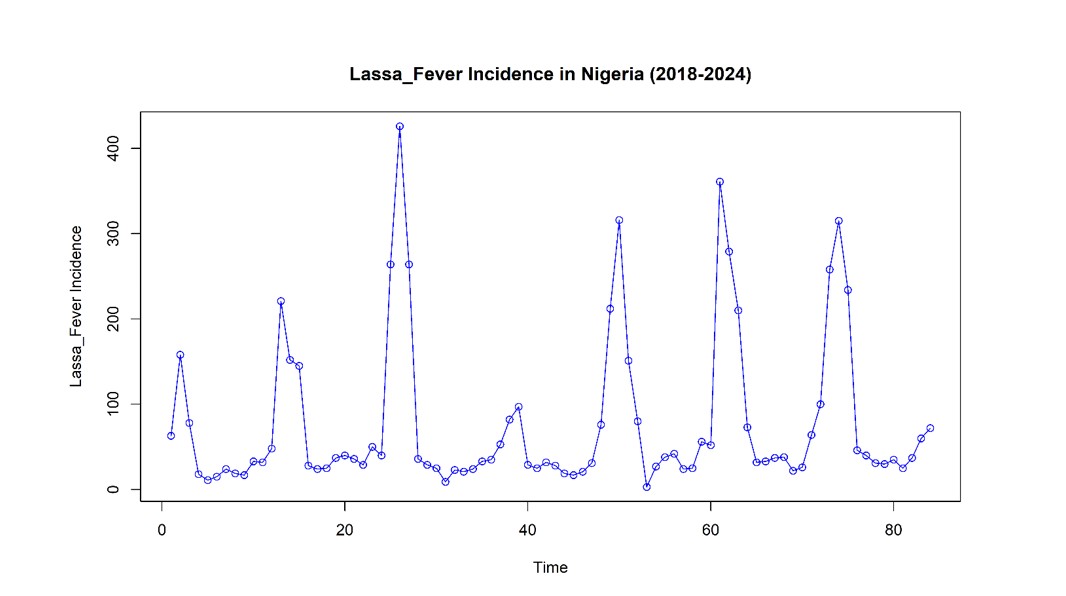
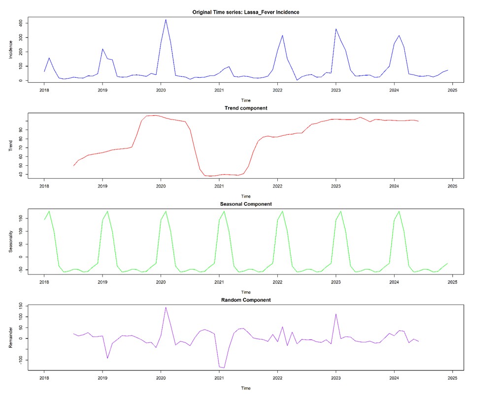
The Augmented Dickey-Fuller test for stationarity yielded a test statistic of −4.8575, with a p-value of 0.01. At the 5% significance level, the null hypothesis of non-stationarity was rejected, confirming that the incidence data is stationary. The Lassa fever incidence data between 2018 to 2024 displayed a largely season and cyclical patterns (Figure 8) with some unique peaks observe once in a year that is accompanied by rapid declines. The decomposition of the time series as shown in Figure 9 revealed a clear trend, a recurring seasonal component, and random noise. The seasonal component focuses on periodic fluctuation of the incidence data, and the random component focuses on residual variation. The ARIMA model, which was fit to the data, has significant seasonal and moving average components with parameters AR (1) = -0.1012, AR (2) = 0.4155, MA (1) = 0.6475, and Seasonal AR (1) = 0.6408.
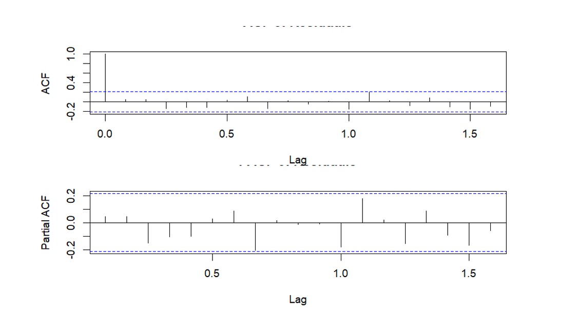
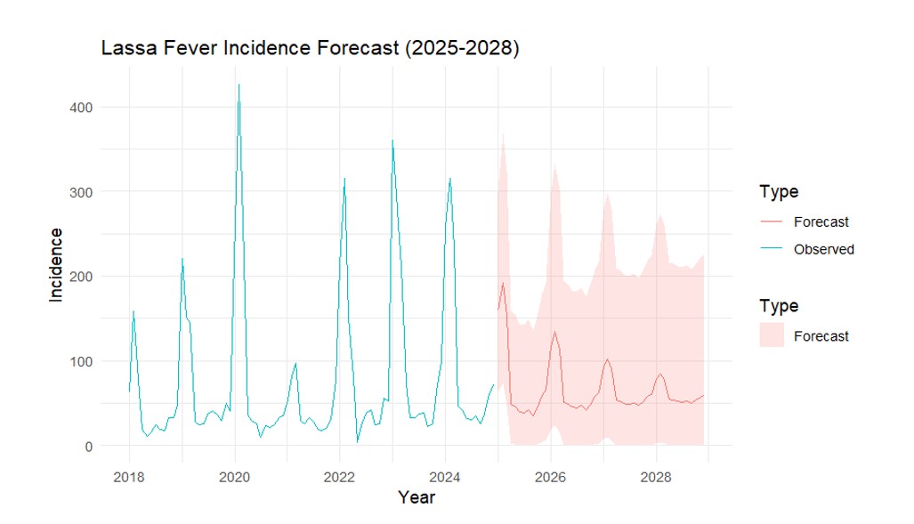
The estimated value for the model intercept was 7.5134. The Box-Ljung test performed on ARIMA residuals produced 21.277 as the test statistic (df = 20, p-value = 0.381). Because the p-value exceeded 0.05 we concluded that the residuals show no signs of autocorrelation. The Lassa Fever incidence data reveals that the ARIMA model successfully captured its time-based patterns and qualifies as an appropriate fit for the data. The fitting of the parameters of the model was estimated as follows: AR (1) = -0.1012, AR (2) = 0.4155, MA (1) = 0.6475, Seasonal AR (1) = 0.6408, and intercept = 7.5134. We selected the parameters of the ARIMA model using the Box–Jenkins approach. The Lag orders for AR, MA, and seasonal components were selected by inspecting the Autocorrelation Function (ACF) and Partial Autocorrelation Function (PACF) plots and confirmed using the lowest AIC and BIC values. The ACF and PACF plots (Figure 10) were checked to assess model adequacy. The absence of spikes outside the 95% confidence intervals indicates no apparent autocorrelation, and thus the ARIMA model has captured the time structure of the data well. The incidence of Lassa Fever for 2025-2028 is projected with expected periodic outbreaks and annual peaks in 2025, 2026, 2027, and 2028, with decreasing intensity compared to previous years. The forecast is paired with 95% prediction intervals, which reflect uncertainty about future incidence rates. The forecast plot (Figure 11) shows the observed incidence along with the forecasted values and confidence levels, showing a rise in cases in certain months.
Hot spot analysis and Lassa fever prevalence mapping
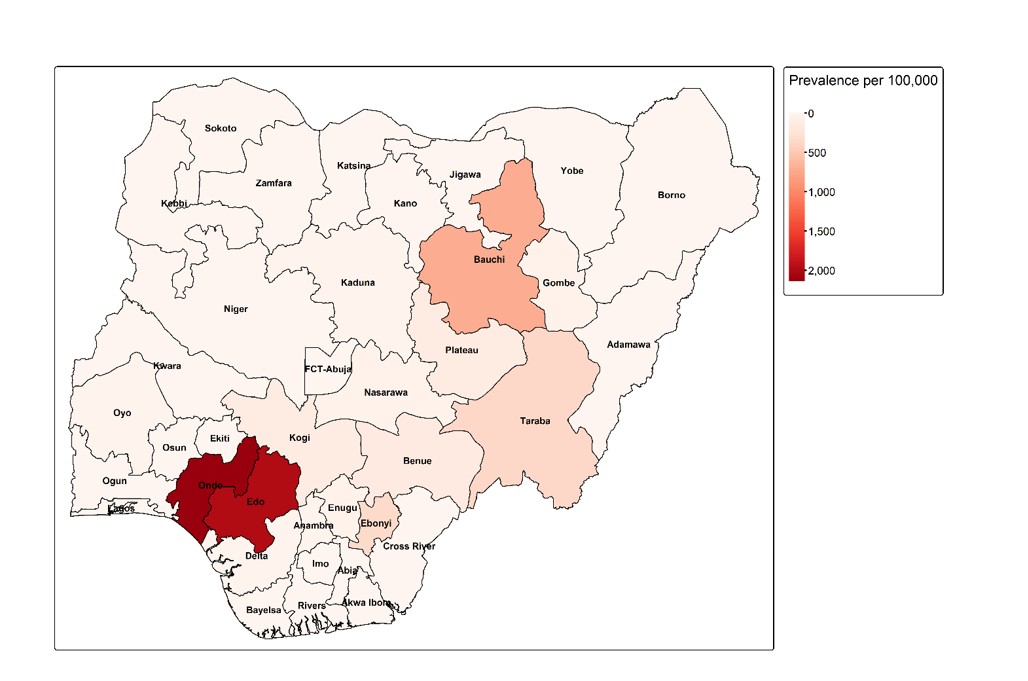
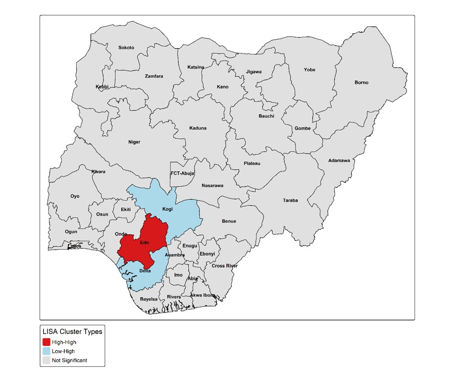
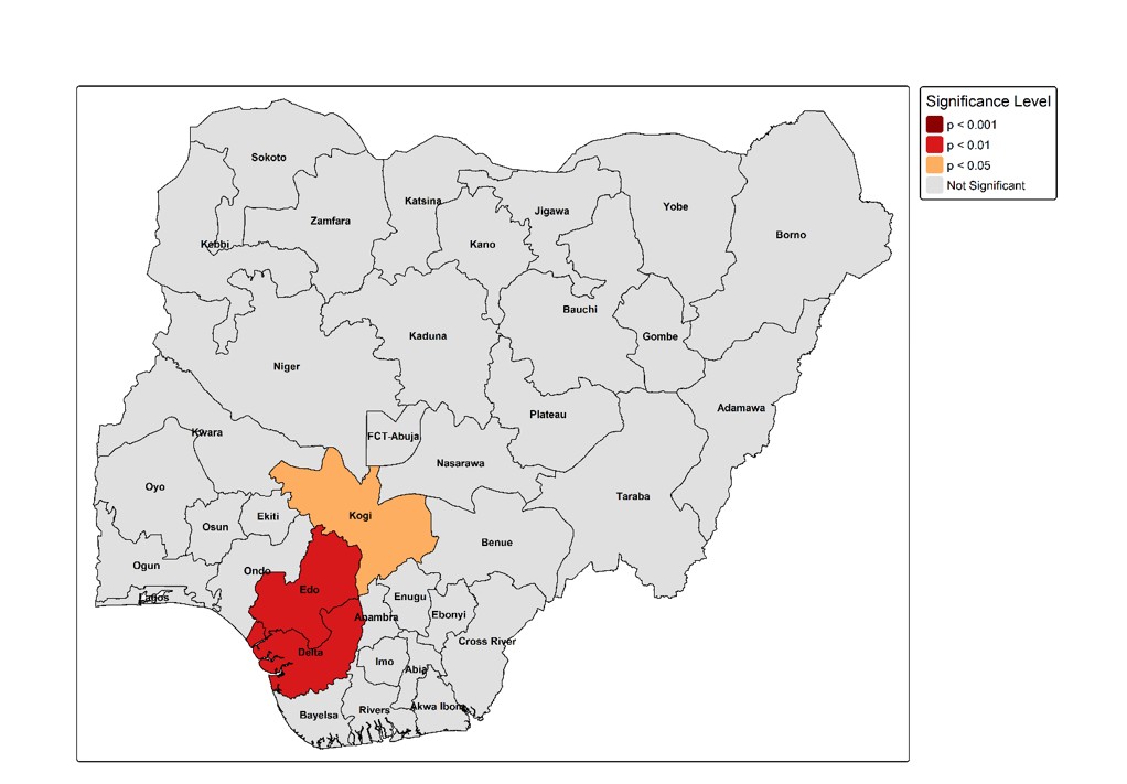
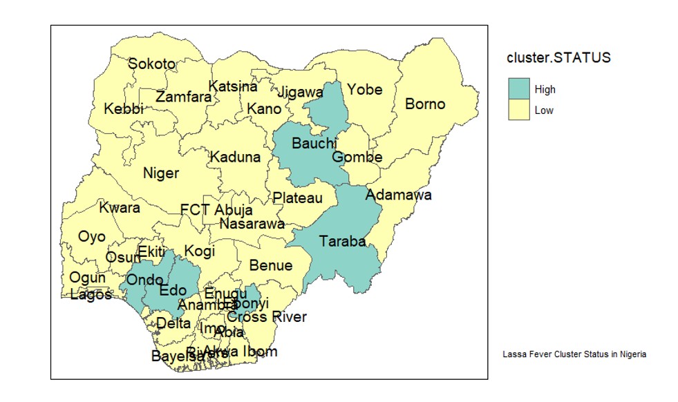
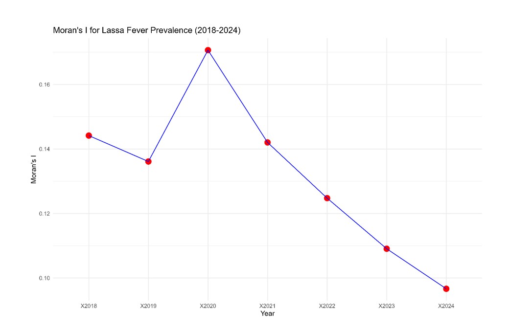
The incidence data revealed on the map some of the states with the highest incidence of Lassa fever, including Ondo, Edo, Kogi, Benue, Ebonyi, Bauchi, Plateau and Taraba states between the years studied, 2018 to 2024 (Figure 12). Hotspots (high-prevalence clusters) were present (Figure 13) in Edo and Delta (p < 0.01), and significant clustering was present in Kogi (p < 0.05). Certain other states, such as Sokoto, Kebbi, Zamfara, Katsina, Ondo, Bauchi, Ebonyi, Ogun, Osun, and Ekiti, also had tendencies for clustering, though they were not all statistically significant. Yobe, Taraba, and Benue did not have any sign of significant clustering. The LISA significance map (Figure 14) displays such clusters in space, where yellow and orange areas represent significant hotspots and grey areas represent non-significant clusters. The Global Moran’s I value was 0.1384 (p = 0.0267), and this was significant at the 5% level. This indicates that the high-prevalence states are locally surrounded by other high-prevalence states and ensures spatial dependence (Figure 15). The results of the spatial regression model indicate that population, primary healthcare coverage, total healthcare coverage, and living conditions, including natural walls and floors, were employed as potential predictors of Lassa fever prevalence. The Ordinary Least Squares (OLS) model possessed a weak R-squared value, indicating that the variables alone are not sufficient to explain the spatial distribution of Lassa fever cases. Additionally, regression residuals were not significantly spatially autocorrelated, according to the Global Moran’s I test, which gave a non-significant result (p = 0.1142). Moran’s I in 2018 was 0.144 (p = 0.014), which showed intense clustering. Clustering was most intense in 2020 (Moran’s I = 0.171, p = 0.008). However, from 2021 onwards, Moran’s I declined gradually and reached 0.097 (p = 0.086) in 2024, and it was not significant. This suggests a decreasing spatial agglomeration of Lassa fever over time, indicating the potential for shifts in its spatial dynamics. Figure 16 illustrates this trend.
The study contributes to our understanding of the spread of Lassa fever in Nigeria by conducting a novel synthesis of compartmental modelling, scenario analysis and spatiotemporal epidemiology. Unlike previous modelling studies on Lassa fever that have focused either on compartmental dynamics [4, 13] or on spatiotemporal patterns [6] in isolation, this work presents a triple-integration framework that combines: (1) a multi-host SEIAR-SEI compartmental model with environmental contamination; (2) geospatial hotspot analysis (Global Moran’s I, LISA); and (3) time series forecasting (ARIMA). This integrated framework reveals a critical discrepancy: while empirical R₀ from incidence data suggests stable endemicity (R_0≈1) , the NGM-derived R_0=1.66 indicates a hidden outbreak potential when zoonotic and environmental pathways are mechanistically modelled. To our knowledge, this is the first study to directly compare three R_0estimation methods (attack rate, incidence, NGM) for Lassa fever in Nigeria and to quantify the substantially higher efficacy of rodent control (61.67% reduction) over healthcare improvement (16.07% reduction) at equivalent implementation levels (25%). The research on R_0 estimates between the years 2018 and 2024 offers important insights into the spread behaviour of both the diseases and the effectiveness of the control measures. Analysis of attack rate and incidence generated consistent low-level endemic transmission data with R_0slightly greater than 1, but Next-Generation Matrix examining the complete transmission pathways of rodent reservoirs through environmental factors generated an R_0 of 1.66. This inconsistency illuminates the possibility of traditional surveillance-based estimates highly underestimating outbreak potential by not accounting for the most important ecological drivers of transmission, which is consistent with other studies of this issue in Sierra Leone [20] and theoretical models of zoonotic diseases [21]. This has significant implications on the preparedness for outbreaks, with the idea that even regions with a history of low-level transmission (R_0 ≈ 1 by incidence measures) can be at significant risk of explosive outbreaks when ecological conditions change. The model possesses two biologically meaningful equilibria. (i) The Disease-Free Equilibrium (DFE), where(E_h,I_Ah,I_Sh,E_r,I_r,C)=(0,0,0,0,0,0)
represents a state of no Lassa fever transmission. The DFE is locally asymptotically stable when R_0 < 1, meaning that small introductions of the virus die out without causing an outbreak. (ii) The Endemic Equilibrium (EE), where all compartments are positive, represents a state of persistent transmission. The EE exists and is stable when R_0> 1. Our estimated R_0= 1.66 > 1 indicates that Nigeria is currently at the endemic equilibrium, where Lassa fever is maintained in both human and rodent populations. The difference between the empirical R_0≈1 and NGM-derived R_0 1.66 suggests that the observed data reflect a system near the DFE due to control efforts, while the true biological potential (in the absence of interventions) is higher.
These transmission dynamics are further explained in the sensitivity analysis, where the human transmission rate β_h, has the strongest positive impact on the R_0, whereas the recovery rates γ_(h )and disease-induced death δ_h have significant negative effects. These findings underline the fact that, although access to healthcare and treatment outcome can help decrease the transmission of Lassa fever, in our scenario analysis, even large (70%) increases in recovery rates had only a 35% effect, whereas similar rodent control interventions had almost twice the effect (58-62% reduction). Such a sharp contrast puts a lot of emphasis on the potential success of interventions aimed at the rodents serving as the reservoir as a way of providing more leverage to the control of the outbreaks as compared to a strategy that focuses on health care interventions [22], but a combination of both approaches is optimal. The particularly high impact of rodent population reduction is consistent with the field research that identifies poor grain storage and housing conditions as major determinants of the Mastomys natalensis proliferation [14, 23].
The analysis of time series shows that there are evident seasonal trends that were identified using the Augmented Dickey-Fuller test, showing stationary periodicity (test statistic = -4.8575, p = 0.01); thus, the stationary periodicity could be used to accurately predict the outbreaks in 2025-2028, with the highest case count of 350. These cyclical variations point to the necessity of interventions with a seasonal schedule, in accordance with studies of climate-related changes in the population of rodents [24, 25]. The time series decomposition into trend, seasonal and residual components will give a useful framework for differentiating between long-term transmission change and periodic changes, as well as random noise.
At the spatial level, our analysis revealed that there is high clustering of the cases (Morans I = 0.1384, p = 0.0267) with consistent hotspots in Sokoto, Kebbi, Edo and Ondo states, which aligns with the past epidemiological surveys [26]. Nevertheless, the decreasing trend in the spatial autocorrelation from 2018 to 2024 indicates a shift in the transmission patterns, potentially indicating improvements in surveillance, disease development, climate-related fluctuations in rodent population or an overall impact of the intervention programs in high-burden regions. This spatial dynamic dimension intensifies the suitability of adaptive surveillance systems that can monitor changing risk patterns over time. The multi-sectoral response can be coordinated, which can contribute to increased efforts to prevent the spread of Lassa fever in Nigeria. High-burden communities could focus on community-led environmental sanitation, including better disposal of waste and rodent-resistant storage of food, especially before seasonal peaks. Enhancement of health systems by increasing diagnostic capacity, having sufficient supplies of essential treatments and practising consistent infection-prevention activities might also help to reduce healthcare-associated transmission.
Surveillance systems can also be useful by shifting towards more action-oriented strategies involving incorporation of findings on rodent population changes and the data on human cases, thus allowing the detection of possible outbreaks early. These efforts could be supplemented with public education campaigns that deal with high-risk behaviours such as unsafe food storage or rodent consumption, which would decrease exposure in the household and community. Policymaking-wise, the results indicate areas that can be applied in prevention-oriented, proactive interventions. To achieve more balanced and sustainable control measures, placing a larger focus on the environmental and zoonotic elements as well as on clinical responses would be helpful. Long-term cost-effectiveness can also be improved by integrating Lassa fever prevention with health-system strengthening and emergency preparedness efforts. On a global level, our finding is consistent with the One Health model, which understands the interrelationship between humans, animals, and the environment in the transmission of zoonotic diseases. The observed spatial clustering decreases with time offers a chance to dig deeper into how long-term interventions could impact the transmission patterns.
Study limitations
This study has several limitations. First, we rely on secondary surveillance data from NCDC, which is subject to underreporting due to limited PCR testing capacity in <30% of Nigerian states [10], potentially biasing incidence estimates downward. Second, our deterministic SEIAR-SEI model assumes homogeneous mixing, which may oversimplify spatial heterogeneity in transmission (though partially addressed by spatial analysis). Third, parameter estimation using nonlinear least squares assumes that residuals are independent and identically distributed, a violation that could affect confidence intervals. Fourth, the rodent population size was assumed proportional to human population (1:1 ratio), whereas actual densities vary spatially with land use and season. Fifth, we did not incorporate climate variables (rainfall, temperature, NDVI) as dynamic drivers of rodent birth rates, which could improve forecast accuracy. Finally, the model does not include human behaviour change (e.g., reduced contact during outbreaks), which may dampen peak incidence in reality
This study integrated spatiotemporal and compartmental modelling to characterise Lassa fever transmission in Nigeria. Three key findings emerge. First, while surveillance data suggests stable endemicity (R_0≈1) , our NGM-derived (R_0=1.66) model incorporating zoonotic and environmental pathways reveals hidden outbreak potential, highlighting that empirical case data alone underestimates risk. Second, rodent population reduction (70% → 61.7% infection reduction) is 3.8-fold more effective than equivalent healthcare improvement (16.1% reduction), demonstrating that reservoir-targeted interventions are epidemiologically superior in this system. Third, persistent spatial hotspots in Edo and Ondo states (Moran’s I=0.138, p=0.027) coupled with seasonal forecasting (peak ~350 cases in 2025-2028) provide actionable windows for seasonally timed, spatially targeted One Health strategies. We conclude that integrated control programs prioritising community-based rodent management alongside healthcare strengthening, timed to seasonal peaks and focused on identified hotspots, offer the most effective pathway for Lassa fever control in Nigeria
Future directions
This study opens several avenues for future research. First, the model can be extended to a stochastic framework to capture the random effects of outbreak ignition in low-transmission regions. Second, climate variables (temperature, rainfall, NDVI) should be incorporated as forcing functions to dynamically modulate rodent birth rates λ_r and transmission rates, potentially improving forecast accuracy. Third, cost-effectiveness analysis should be performed to compare the economic trade-offs between rodent control campaigns (e.g., community-based sanitation, rodenticides) and healthcare system strengthening (e.g., ribavirin stockpiles, PPE). Fourth, the model could be adapted to other West African countries (Sierra Leone, Guinea, Liberia) to test the generalizability of the R_0=1.66 finding. Finally, if vaccine candidates become available, the SEIAR framework can be modified to include a vaccination compartment (V_h ) to evaluate herd immunity thresholds
What is already known about the topic
What this study adds
This research was funded by the Bill & Melinda Gates Foundation [Grant number INV-048039]. The funders had no role in data analysis, the decision to publish, or the preparation of the manuscript.
Abbreviations
ACF: Autocorrelation Function
ADF: Augmented Dickey-Fuller
AIC: Akaike Information Criterion
AR: Autoregressive
ARIMA: Autoregressive Integrated Moving Average
BIC: Bayesian Information Criterion
CFR: Case Fatality Rate
DFE: Disease-Free Equilibrium
EE: Endemic Equilibrium
IDSR: Integrated Disease Surveillance and Response
LASV: Lassa virus
LISA: Local Indicators of Spatial Association
MA: Moving Average
MAPE: Mean Absolute Percentage Error
MICS: Multiple Indicator Cluster Survey
NBS: National Bureau of Statistics
NCDC: Nigeria Centre for Disease Control
NGM: Next-Generation Matrix
ODE: Ordinary Differential Equation
OLS: Ordinary Least Squares
PACF: Partial Autocorrelation Function
PCR: Polymerase Chain Reaction
R₀: Basic Reproduction Number
RK4: Fourth-Order Runge-Kutta
RMSE: Root Mean Square Error
RT-PCR: Reverse-Transcription Polymerase Chain Reaction
SEI: Susceptible-Exposed-Infectious (rodent model)
SEIAR: Susceptible-Exposed-Asymptomatic-Symptomatic-Recovered (human model)
Conceptualization: Polycarp Dauda Madaki, Chijioke Kaduru
Methodology: Polycarp Dauda Madaki, Oghenetega ThankGod Oweh, Zubairu Dalhatu Zubairu, Charles Obi
Funding acquisition: Chijioke Kaduru
Data curation: Polycarp Dauda Madaki, Sylvia Adanma Ezenwa-Ahanene, Charles Obi
Formal analysis: Polycarp Dauda Madaki
Investigation: Polycarp Dauda Madaki
Validation: Olalekan Taiwo, Zubairu Dalhatu Zubairu, Charles Obi, Oghenetega ThankGod Oweh, Dupsy Akoma
Supervision: Chijioke Kaduru, Olalekan Taiwo, Charles Obi
Project administration: Ganiyat Eshikhena
Writing- original draft: Polycarp Dauda Madaki, Oghenetega ThankGod Oweh, Ezra Gayawan
Writing – review & editing: Polycarp Dauda Madaki, Oghenetega ThankGod Oweh, Dupsy Akoma, Ruth Manzo Sabo, Zainab Dambazau, Jide Idris, Oladipo Ogunbode, Chijioke Kaduru
| Parameter | Description | Values-1 | Units | Reference |
|---|---|---|---|---|
| λₕ | Recruitment rate of humans | 0.34 | week⁻¹ | Estimated |
| βₕᵣ | Transmission rate from rodents to humans | 0.0509 | week⁻¹ | Fitted |
| βₕₕ | Transmission rate from humans to humans | 0.196 | week⁻¹ | Fitted |
| βₑᵥ | Transmission rate from environment to humans | 0.028 | week⁻¹ | Fitted |
| μₕ | Natural death rate of humans | 0.00133 | week⁻¹ | Estimated |
| P | Proportion of asymptomatic infections | 0.8 | dimensionless | [13] |
| σₕ | Progression rate from exposed to infectious | 0.16136 | week⁻¹ | Fitted |
| γₕ | Recovery rate of humans | 0.1122 | week⁻¹ | Fitted |
| δₕ | Disease-induced death rate in humans | 0.0189 | week⁻¹ | [9] |
| ωₕ | Rate of immunity loss in humans | 0.03278 | week⁻¹ | [4] |
| λᵣ | Recruitment rate of rodents | 0.05 | week⁻¹ | [27] |
| βᵣᵣ | Transmission rate among rodents | 0.0254 | week⁻¹ | [17][27] |
| μᵣ | Natural death rate of rodents | 0.0192 | week⁻¹ | Estimated |
| σᵣ | Progression rate in rodents | 0.004 | week⁻¹ | [4] |
| Η | Contamination rate by infected rodents | 0.046 | week⁻¹ | Estimated |
| Ξ | Clearance rate of the environment | 0.078 | week⁻¹ | [28] |
| Parameter | Description | Sensitivity Index | Interpretation |
|---|---|---|---|
| βhh | Human-to-human transmission rate | + 1.00 | A 1% increase in βhh increases R0 by 1% (strongest positive driver) |
| γh | Human recovery rate | – 0.73 | A 1% increase in γh decreases R0 by 0.73% (strongest negative driver) |
| δh | Disease-induced death rate | – 0.246 | A 1% increase in δh decreases R0 by 0.246% |
| σh | Progression rate (exposed → infectious) | + 0.0207 | Negligible positive effect |
| μh | Natural death rate of humans | – 0.04 | Negligible negative effect |