
Review | Open Access | Volume 9 (3): Article 153 | Published: 24 Sep 2026

Views: 62
Menu, Tables and Figures
Table 1. Quality assessment results for included studies (n = 40)
| Quality domain | High quality n (%) | Moderate quality n (%) | Low quality n (%) |
|---|---|---|---|
| Clarity of methodological presentation | 28 (70.0) | 9 (22.5) | 3 (7.5) |
| Theoretical depth and mathematical rigor | 24 (60.0) | 12 (30.0) | 4 (10.0) |
| Comprehensiveness of coverage | 21 (52.5) | 15 (37.5) | 4 (10.0) |
| Appropriateness of conclusions | 31 (77.5) | 7 (17.5) | 2 (5.0) |
| Practical utility for applied researchers | 19 (47.5) | 14 (35.0) | 7 (17.5) |
Table 1: Quality assessment results for included studies (n = 40)
Table 2: Comparison of count data models
| Model | Distribution | Handles overdispersion | Handles underdispersion | Handles Zero Inflation | Handles correlation | Key limitations / features |
|---|---|---|---|---|---|---|
| Poisson | Poisson | No | No | No | No | Equidistribution assumption |
| Negative Binomial | NB | Yes | No | No | No | Does not handle underdispersion |
| Generalized Poisson | GP | Yes | Yes | No | No | Complicated likelihood function |
| ZIP | Poisson | Yes (from zeros) | No | Yes | No | Does not handle structural overdispersion |
| ZINB | NB | Yes | No | Yes | No | Computationally intensive |
| Hurdle | Truncated count | Yes | No | Yes | No | Assumes separate processes |
| Quasi-Poisson | Quasi-likelihood | Yes | No | No | No | Not a true likelihood function |
| Conway-Maxwell-Poisson | CMP | Yes | Yes | No | No | Normalizing constant is computationally complex |
| GEE | Quasi-likelihood | Yes | No | No | Yes | Requires large sample size |
| Panel/Random Effects | Varies | Yes | No | No | Yes | Computationally intensive |
Table 2: Comparison of count data models
Kare Chawicha Debessa¹,&
1School of Public Health, College of Medicine and Health Sciences, Hawassa University, Hawassa, Ethiopia
&Corresponding author: Kare Chawicha Debessa, School of Public Health, College of Medicine and Health Sciences, Hawassa University, Hawassa, Ethiopia, Email: kare.debessa@gmail.com, ORCID: https://orcid.org/0009-0002-6118-9153
Received: 20 Jun 2026, Accepted: 20 Jun 2026, Published: 24 Sep 2026
Domain: Medical Statistics
Keywords: Count data, poisson regression, negative binomial, zero-inflated models, urdle models, overdispersion, zero inflation, model diagnostics
©Kare Chawicha Debessa. Journal of Interventional Epidemiology and Public Health (ISSN: 2664-2824). This is an Open Access article distributed under the terms of the Creative Commons Attribution International 4.0 License (https://creativecommons.org/licenses/by/4.0/), which permits unrestricted use, distribution, and reproduction in any medium, provided the original work is properly cited.
Cite this article: Kare Chawicha Debessa, A narrative review of count data models. Journal of Interventional Epidemiology and Public Health. 2026; 9(3):153. https://doi.org/10.37432/jieph-d-26-00263
Introduction: Count data represent the frequency of event occurrences; therefore, they are inherently discrete and non-negative. Modelling such data presents considerable challenges when excessive zeros exist or when variability exceeds expected levels. Standard linear regression approaches are inappropriate for these data types. This narrative review examined principal models for count data analysis, beginning with foundational approaches and progressing to advanced methods that address overdispersion, zero inflation, and unobserved heterogeneity.
Methods: A systematic literature search was conducted across PubMed, Scopus, Web of Science, and Google Scholar for articles published between 2000 and 2026. The search strategy employed keywords including “count data,” “Poisson regression,” “Negative Binomial,” “zero-inflated models,” “hurdle models,” “overdispersion,” and “zero inflation.” I included studies that addressed methodological developments, comparative evaluations, or applications of count data models. Data extraction focused on model specifications, estimation procedures, diagnostic approaches, and practical recommendations.
Results: The review identified that Poisson regression serves as the foundational approach; however, the equidispersion assumption often fails in practice. The Negative Binomial model addresses overdispersion through an additional dispersion parameter. Generalized Poisson models provide flexibility for both over- and underdispersion. Zero-Inflated Poisson and Zero-Inflated Negative Binomial models combine a point mass at zero with a count process. Hurdle models treat zeros and positive counts as separate outcomes. Advanced methods include finite mixture models and panel count models with random effects. Estimation techniques such as maximum likelihood and the expectation maximization algorithm are widely employed. Diagnostic tools including residual analysis, overdispersion tests, and zero-inflation tests are essential for model evaluation.
Conclusions: This review provides researchers with a clear guide to the theory, methods, and applications of count data models across various disciplines. Proper model specification, estimation, and diagnostic evaluation are essential for valid inference.
Count data are ubiquitous in empirical research because they capture the number of times an event occurs within a specified period, area, or context. These data are discrete and non-negative; consequently, standard linear regression models that assume continuous outcomes are inappropriate for count data analysis [1]. The classical approach to modelling count data is Poisson regression, which assumes that the count variable follows a Poisson distribution. This model relies on the equidispersion assumption, meaning that the distribution’s mean and variance are equal. The Poisson model is mathematically elegant and computationally straightforward; therefore, it serves as a starting point for count data analysis [2].
Empirical datasets often violate the equidispersion assumption. Overdispersion, where the variance exceeds the mean, is a common phenomenon caused by unobserved heterogeneity, omitted variables, or clustering effects [3]. When overdispersion is present, the Poisson model underestimates the variance; therefore, it produces underestimated standard errors, inflated test statistics, and potentially misleading inferences [4]. To address this limitation, the Negative Binomial (NB) model introduces an additional dispersion parameter, which allows the variance to exceed the mean. The NB model can be viewed as a Poisson-gamma mixture, where the count follows a Poisson distribution and the rate parameter follows a gamma distribution; consequently, it accommodates overdispersion [5].
Beyond the NB model, the Generalized Poisson distribution offers further flexibility by allowing for both overdispersion and underdispersion. This distribution modifies the Poisson probability mass function with an additional parameter, thereby enabling the modeling of a wider range of data variability [6]. These models are estimated via maximum likelihood estimation; consequently, their parameters are typically obtained through iterative algorithms such as Newton–Raphson or Fisher scoring [7].
Some data exhibit an excess of zeros beyond what standard count models can accommodate [8]. Zero inflation arises when structural reasons for zeros exist; for example, individuals who are not at risk of experiencing the event at all. To model such data, zero-inflated models were developed [8]. These models assume that the data-generating process comprises two parts: a binary process that determines whether an observation is always zero and a count process that generates counts and can also produce zeros. The Zero Inflated Poisson combines a logistic model for the zero-inflation component with a Poisson count model (ZIP) model [9]. In contrast, the Zero Inflated Negative Binomial (ZINB) extends this approach by using the NB distribution for the count component. These models are estimated via maximum likelihood, and the Expectation Maximization (EM) algorithm is often used to handle the mixture structure [10].
Hurdle models offer an alternative approach for zero-inflated data. Unlike zero-inflated models, they assume that zeros and positive counts arise from separate processes. Zero counts are modeled with a binary process, typically logistic regression, and positive counts are modeled with a truncated count distribution that excludes zeros. This two-part structure provides greater flexibility, especially when the zero and positive processes are believed to be driven by different mechanisms [11].
Advanced frameworks have been developed to handle heterogeneity and longitudinal data structures. Finite mixture models treat the population as a mixture of subpopulations, each with its own count distribution; these models capture unobserved heterogeneity [12]. Panel count models incorporate random effects to account for correlation across repeated observations within individuals or groups; these models are often implemented via hierarchical Bayesian methods or marginal models with random effects [13].
Model fitting involves specifying likelihood functions derived from the assumed distributions and estimating parameters through maximum likelihood or Bayesian methods [14]. Diagnostic tools such as residual analysis, goodness-of-fit tests, and tests for overdispersion or zero inflation are crucial for evaluating model adequacy. For example, the Vuong test can compare non-nested models such as ZIP versus Poisson, while overdispersion tests help determine whether the NB model is more appropriate than the Poisson model [15]. In practice, the choice of model depends on data characteristics and the underlying data-generating process. Proper model specification, estimation, and diagnostic evaluation are essential for valid inference [16].
Search strategy
This single-author methodological review was conducted as a narrative review. Selected PRISMA reporting principles were used to improve transparency in the search and selection process; however, because the manuscript has one author, duplicate independent screening and formal systematic-review status were not applicable. A structured literature search was conducted across four electronic databases: PubMed, Scopus, Web of Science, and Google Scholar. The search was restricted to articles published between January 2000 and August 2026. The search strategy employed combinations of keywords and Medical Subject Headings (MeSH) terms, including: “count data,” “Poisson regression,” “Negative Binomial regression,” “Generalized Poisson,” “zero-inflated models,” “hurdle models,” “overdispersion,” “zero inflation,” “finite mixture models,” “panel count models,” “maximum likelihood estimation,” and “model diagnostics.” The Boolean operators “AND” and “OR” were used to combine search terms. Additionally, the reference lists of included articles were manually screened to identify additional relevant studies.
Inclusion and exclusion criteria
Studies were included if they met the following criteria: (a) addressed methodological developments or comparative evaluations of count data models; (b) provided theoretical foundations, estimation procedures, or diagnostic approaches; (c) were published in peer-reviewed journals; (d) were written in English. Studies were excluded if they: (a) focused exclusively on software implementation without methodological discussion; (b) were conference abstracts or dissertations; (c) did not address count data modelling specifically; (d) were not available in full text.
Study selection and data extraction
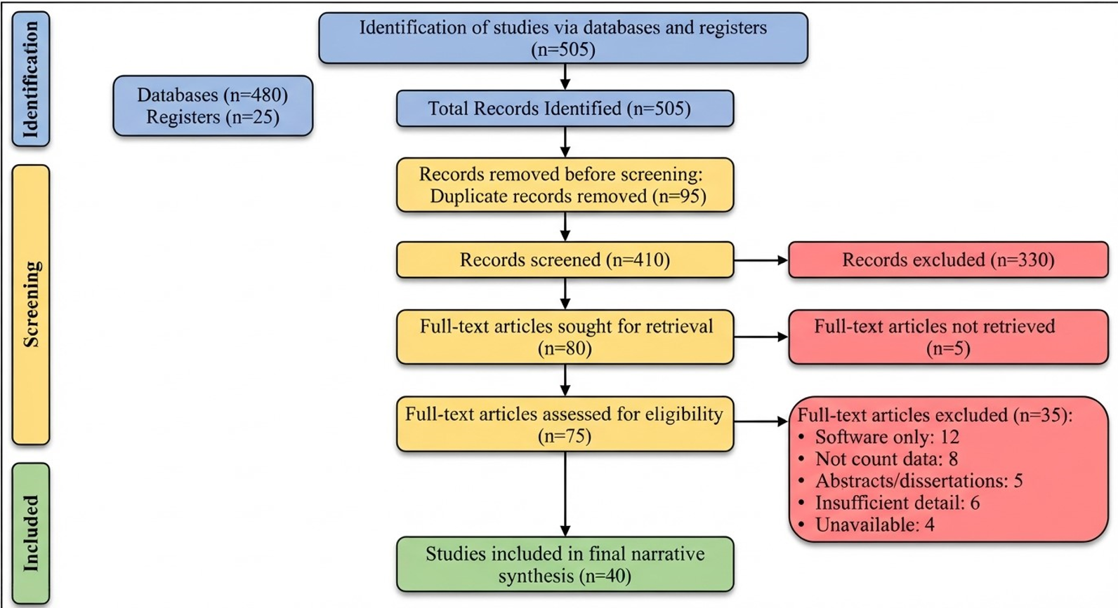
Figure 1 presents a PRISMA-style flow diagram of the study selection process. The search identified 505 records (480 from databases, 25 from references). Subsequently, 95 duplicates were removed. Then, 410 records underwent title and abstract screening. Of these, 330 records were excluded. Thus, 80 full texts were sought for retrieval. However, five were not retrieved. Therefore, 75 full texts were assessed for eligibility. Specifically, 35 studies were excluded due to software only (n=12), not count data (n=8), abstracts or dissertations (n=5), insufficient detail (n=6), and unavailability (n=4). Ultimately, 43 studies met the inclusion criteria for the final narrative synthesis (Figure 1).
The author independently screened all titles and abstracts. Because this was a single-author narrative review, no second independent reviewer was available. Therefore, consensus procedures for disagreements were not applicable. Data extraction was performed using a standardized form. This form captured model specifications and assumptions, estimation procedures, diagnostic methods, comparative findings, practical recommendations, and identified limitations and challenges.
Quality assessment
The quality of the 43 included studies was assessed. The author used adapted criteria. These criteria were suitable for a methodological review. Most included sources were methodological papers, simulation studies, or applied analyses. They were not clinical trials or observational epidemiological studies. The assessment covered five domains. These domains were clarity of methodological presentation, theoretical depth and mathematical rigour, comprehensiveness of coverage, appropriateness of conclusions, and practical utility for applied researchers. Each domain was rated as high, moderate, or low quality.
A study was rated high quality if it met several criteria. These criteria were complete mathematical derivations, clear model assumptions, simulation or empirical validation, and practical implementation guidance. A study was rated moderate quality if it addressed key methodological concepts. However, it lacked full technical detail or empirical validation. A study was rated low quality if it provided superficial coverage. Moreover, it lacked adequate theoretical foundation or practical guidance.
Table 1 presents the quality assessment results. Overall, 26 studies (60.5%) were high quality. 13 studies (30.2%) were moderate quality. 4 studies (9.3%) were low quality. The strongest domain was appropriateness of conclusions. In this domain, 31 studies (72.1%) were high quality. The second strongest domain was clarity of methodological presentation. In this domain, 28 studies (65.1%) were high quality. The weakest domain was practical utility for applied researchers. In this domain, only 19 studies (44.2%) were high quality. This weakness reflects a common limitation. Many methodological papers provide theoretical developments (Table 1). However, they do not provide software code, worked examples, or implementation guidance.
Low-quality studies focused narrowly on a single model application. Moreover, they lacked comparative evaluation or diagnostic assessment. These studies were retained in the narrative synthesis. They provided illustrative applications in specific disciplinary contexts. Nevertheless, their methodological contributions were weighted less heavily. High-quality studies were weighted more heavily. Consequently, practical recommendations came mainly from high-quality studies.
This was a single-author narrative review. Therefore, no second independent reviewer was available. As a result, quality assessment could not be duplicated. Discrepancies could not be resolved through consensus. To mitigate bias, the author rechecked all full texts against the quality criteria. In addition, the author applied the criteria consistently across studies. The absence of duplicate independent quality assessment remains a limitation. This limitation should be considered when interpreting the findings.
The quality of included methodological reviews was assessed by the author using adapted criteria, including clarity of presentation, theoretical depth, comprehensiveness of coverage, and appropriateness of conclusions. Because no second reviewer was involved, discrepancies were not resolved through consensus; instead, the author rechecked the full texts and applied the criteria consistently.
Data synthesis
A narrative synthesis approach was employed due to the heterogeneity of study designs and outcomes. Findings were organized thematically around model types, estimation approaches, diagnostic tools, and practical recommendations. Mathematical formulations and comparative tables were constructed to facilitate understanding of model relationships and selection.
Foundational count data models
Poisson regression model
The Poisson regression model serves as the fundamental approach for count data analysis. For a response variable Yᵢ, the Poisson distribution has the probability mass function:
P(Yᵢ = yᵢ | μᵢ) = exp(-μᵢ) μᵢ^(yᵢ) / yᵢ!
where yᵢ = 0, 1, 2, … and μᵢ > 0 is the expected count. The Poisson distribution has the property that E(Yᵢ) = Var(Yᵢ) = μᵢ, which constitutes the equidispersion assumption. The log-linear link function relates the expected count to the linear predictor:
log(μᵢ) = β₀ + β₁xᵢ₁ + β₂xᵢ₂ + … + βₚxᵢₚ
where β are regression coefficients, and x are covariates. Maximum likelihood estimation is used to obtain parameter estimates [17]. The log-likelihood function for independent observations is:
l(β) = Σᵢ [yᵢ log(μᵢ) – μᵢ – log(yᵢ!)]
The model’s computational simplicity and interpretability make it appealing for initial count data analysis; however, the equidispersion assumption often fails in practice, necessitating more flexible approaches [18].
Negative binomial regression model
The Negative Binomial (NB) model addresses overdispersion by introducing an additional dispersion parameter. The NB distribution can be derived as a Poisson-gamma mixture. The probability mass function is:
P(Yᵢ = yᵢ | μᵢ, θ) = Γ(yᵢ + θ) / (Γ(θ) yᵢ!) × (θ / (θ + μᵢ))^θ × (μᵢ / (θ + μᵢ))^yᵢ
where θ > 0 is the dispersion parameter. This mixture yields a variance structure where Var(Yᵢ) = μᵢ + μᵢ²/θ, which exceeds the mean. As θ → ∞, the NB distribution approaches the Poisson distribution. The NB model maintains the same log-linear link function as Poisson regression [19].
Generalized poisson model
The Generalized Poisson (GP) distribution provides additional flexibility by accommodating both overdispersion and underdispersion [20]. The probability mass function is:
P(Yᵢ = yᵢ | μᵢ, λ) = (μᵢ / (1 + λ μᵢ))^yᵢ × (1 + λ yᵢ)^(yᵢ-1) / yᵢ! × exp[-μᵢ(1 + λ yᵢ)/(1 + λ μᵢ)]
where λ is the dispersion parameter. When λ = 0, the GP distribution reduces to the Poisson distribution; when λ > 0, it exhibits overdispersion; and when -1/μ < λ < 0, it exhibits underdispersion. This parameterization allows the GP model to serve as a unified framework for count data with varying dispersion patterns [21].
Offset and exposure adjustment
Count data often arise from observation units with differing exposure sizes, such as person-time, population size, area, or number of trials [22]. When exposure varies across observations, the expected count should be modelled relative to exposure rather than as an absolute count. This is accomplished by including an offset variable in the linear predictor [23]. For the Poisson model, the log-linear link becomes: log(μᵢ) = log(tᵢ) + β₀ + β₁xᵢ₁ + β₂xᵢ₂ + … + βₚxᵢₚ where tᵢ is the known exposure or offset for observation i. Equivalently, the model can be written as: log (μᵢ / tᵢ) = β₀ + β₁xᵢ₁ + β₂xᵢ₂ + … + βₚxᵢₚ The coefficient of log(tᵢ) is fixed at 1 rather than estimated as an ordinary regression coefficient. Offset variables are used in the same way for Negative Binomial, Generalized Poisson, zero-inflated, hurdle, and other count regression models, because the offset adjusts the expected count for differential exposure while the covariate effects are estimated on the rate scale [24]. Failure to include an appropriate offset when exposure varies can bias estimated covariate effects and lead to misleading inference [25].
Models for zero-inflated count data
Zero-inflated Poisson model
The Zero-Inflated Poisson (ZIP) model addresses excess zeros in count data by assuming that the data arise from a mixture of two distributions. The probability mass function is: P(Yᵢ = yᵢ | πᵢ, μᵢ) = πᵢ + (1 – πᵢ) exp(-μᵢ), if yᵢ = 0 P(Yᵢ = yᵢ | πᵢ, μᵢ) = (1 – πᵢ) exp(-μᵢ) μᵢ^(yᵢ) / yᵢ!, if yᵢ > 0
where πᵢ represents the probability of belonging to the zero state (i.e., the observation is structurally zero). The zero-inflation probability can depend on covariates through a logistic model:
logit(πᵢ) = γ₀ + γ₁zᵢ₁ + … + γₘzᵢₘ,
while the count component uses a log-linear model. The ZIP model accommodates overdispersion arising from excess zeros [26].
Zero-inflated negative binomial model
The Zero-Inflated Negative Binomial (ZINB) model extends the ZIP framework by using an NB distribution for the count component. The probability mass function is:
P(Yᵢ = 0 | πᵢ, μᵢ, θ) = πᵢ + (1 – πᵢ) (θ / (θ + μᵢ))^θ
P(Yᵢ = yᵢ | πᵢ, μᵢ, θ) = (1 – πᵢ) Γ(yᵢ + θ) / (Γ(θ) yᵢ!) × (θ / (θ + μᵢ))^θ × (μᵢ / (θ + μᵢ))^yᵢ, for yᵢ > 0
The ZINB model provides greater flexibility than ZIP because it accommodates both excess zeros and overdispersion simultaneously through inclusion of both a zero-inflation parameter and a dispersion parameter. This dual capability makes the ZINB model particularly suitable for datasets where both sources of variability are present [27].
Hurdle models
Hurdle models consist of two parts: a binary process determining whether the count is zero or positive, and a truncated count process for positive observations. The probability mass function is: P(Yᵢ = 0) = φᵢ
P(Yᵢ = yᵢ) = (1 – φᵢ) P(Y = yᵢ | y > 0), for yᵢ > 0
where φᵢ is the hurdle probability. The positive counts are modeled with a count distribution truncated to exclude zeros [28]. For a Poisson hurdle model, the positive part is: P(Y = y | y > 0) = exp(-μ) μ^y / (y! (1 – exp(-μ)))
Hurdle models differ from zero-inflated models in their interpretation: zeros in hurdle models arise from a single process (the hurdle), whereas zeros in zero-inflated models arise from two possible processes. This distinction has important implications for model selection and interpretation, particularly when the mechanisms generating zeros are of substantive interest [11].
Advanced models
Finite mixture models
Finite mixture models capture unobserved heterogeneity by assuming the population consists of multiple latent subpopulations, each with its own count distribution. The overall distribution is:
f(yᵢ | Θ) = Σ_{k=1}^K π_k f_k(yᵢ | θ_k)
where K is the number of components, π_k are mixing proportions (0 < π_k < 1, Σπ_k = 1), and f_k are component distributions from the exponential family [29]. The mixture model provides flexible modeling of complex distributions and can accommodate multiple modes and other non-standard features. This flexibility makes finite mixture models valuable for exploring latent structures in count data, though they require careful specification of the number of components and are computationally intensive [30].
Panel count models with random effects
Panel count models account for correlation across repeated observations within individuals or groups by incorporating random effects into the linear predictor. The mixed-effects framework adds subject-specific terms that capture within-subject correlation:
log(μᵢⱼ) = β₀ + β₁xᵢⱼ₁ + … + βₚxᵢⱼₚ + bᵢ
where bᵢ ~ N(0, σ²) are random effects [31]. The model accommodates both overdispersion and correlation among repeated measures, making it appropriate for longitudinal count data. Estimation is often performed using numerical integration techniques or through Bayesian hierarchical approaches [32].
Estimation methods
Maximum likelihood estimation
Maximum likelihood estimation (MLE) is the primary approach for parameter estimation in count data models. The log-likelihood function is specified based on the assumed distribution. For the Poisson model, the log-likelihood is: l(β) = Σᵢ [yᵢ log(μᵢ) – μᵢ – log(yᵢ!)] Parameter estimates are obtained by maximising the log-likelihood function, typically using iterative numerical optimization algorithms. MLE provides consistent and asymptotically efficient estimates under regularity conditions; furthermore, it provides a framework for constructing confidence intervals and hypothesis tests based on the asymptotic normality of the estimators [33].
Expectation maximization algorithm
The Expectation Maximization (EM) algorithm is particularly useful for mixture models and zero-inflated models where the likelihood function involves latent variables. The algorithm alternates between two steps: Expectation Step (E-step): Compute the expected complete-data log-likelihood conditioning on observed data and current parameter estimates:
Q(θ | θ^(t)) = E[log L(θ | Y, Z) | Y, θ^(t)]
where Z represents latent variables (e.g., component membership indicators in mixture models or zero-state indicators in ZIP models). Maximization Step (M-step): Maximize the expected complete-data log-likelihood to obtain updated parameter estimates:
θ^(t+1) = argmax Q(θ | θ^(t))
The EM algorithm provides stable convergence and naturally handles missing data structures, including latent class memberships and zero-inflation indicators [34]. Although convergence can be slow, the EM algorithm is widely used because each maximization step typically has a closed-form solution or involves simple standard estimation procedures [35].
Model diagnostics and selection Residual analysis
Residual analysis provides critical information about model fit and helps identify violations of model assumptions. For count data models, Pearson residuals are defined as:
r_i = (yᵢ – μ̂ᵢ) / √Var(Yᵢ)
Deviance residuals are defined as:
d_i = sign(yᵢ – μ̂ᵢ) √{2 [yᵢ log(yᵢ / μ̂ᵢ) – (yᵢ – μ̂ᵢ)]}
Randomized quantile residuals are often preferred for their improved performance in detecting model misspecification. These residuals transform the data to approximate normality, thereby facilitating standard diagnostic procedures [36].
Overdispersion tests
Tests for overdispersion help determine whether the NB model is more appropriate than the Poisson model. Common approaches include:
Likelihood Ratio Test (LRT): Compares the log-likelihood of the Poisson model (constrained, θ = 0) against the NB model (unconstrained). The test statistic is: LR = 2(l_NB – l_Poisson) which follows a mixture of chi-square distributions.
Score test: Assesses whether the dispersion parameter significantly differs from zero without estimating the alternative model [37].
Wald test: Evaluates the significance of the dispersion parameter using: W = θ̂² / Var(θ̂) These tests are important because selecting a model that incorrectly assumes equidispersion can lead to invalid inference, while using an overdispersed model when not needed may result in a loss of efficiency [38].
Zero-inflation tests
Tests for zero-inflation help determine whether zero-inflated models are necessary. The Vuong test is commonly used for comparing non-nested models such as ZIP versus Poisson. The test statistic is:
Vuong = (1/√n) Σᵢ log[f₁(yᵢ | xᵢ) / f₂(yᵢ | xᵢ)] / SD[log(f₁/f₂)]
where f₁ and f₂ are the probability mass functions of the competing models [39]. Positive values favor the zero-inflated model. Other approaches include score tests and information criteria such as AIC and BIC, which can be used to compare nested and non-nested models [40].
Additional count regression approaches
Quasi-Poisson regression
Quasi-Poisson regression addresses overdispersion by introducing a dispersion parameter φ into the variance function: Var(Yᵢ) = φ μᵢ where φ > 0 is estimated from the data. This approach does not specify a full probability distribution; instead, it uses quasi-likelihood estimation. The regression coefficients are estimated identically to Poisson regression; however, standard errors are multiplied by √φ to account for overdispersion. Quasi-Poisson is computationally simple and provides robust inference; nevertheless, it does not provide a likelihood for model comparison [41].
Conway-maxwell-poisson regression
The Conway-Maxwell-Poisson (CMP) distribution generalizes the Poisson distribution by adding a dispersion parameter ν that controls the rate of decay of successive probabilities. The probability mass function is:
P(Y = y) = (λ^y) / ((y!)^ν Z(λ, ν))
where Z(λ, ν) = Σ_{j=0}^∞ λ^j / (j!)^ν is a normalizing constant. When ν = 1, the CMP reduces to the Poisson distribution; when ν < 1, it accommodates overdispersion; when ν > 1, it accommodates underdispersion. This model provides a unified framework for modeling count data with varying dispersion patterns [42].
Generalized estimating equations
Generalized Estimating Equations (GEE) extend generalized linear models to correlated count data. The estimating equations are:
Σᵢ Dᵢᵀ Vᵢ⁻¹ (yᵢ – μᵢ) = 0
where Dᵢ = ∂μᵢ/∂β, Vᵢ = Aᵢ^(1/2) R(α) Aᵢ^(1/2) is the working covariance matrix, Aᵢ is a diagonal matrix of variance functions, and R(α) is a working correlation matrix. GEE provides consistent estimates even when the correlation structure is misspecified; however, inference depends on robust standard errors [43].
Model selection framework
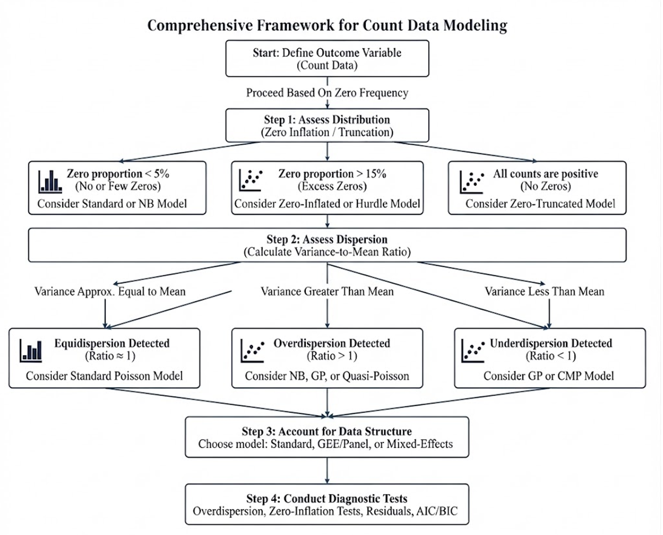
As outlined in Figure 2, the methodological decision framework for count data modeling follows a structured, sequential workflow. First, Step 1 involves assessing the distribution of the outcome variable: if there are no or few zeros (zero proportion < 5%), Poisson or negative binomial (NB) models are considered; if there are excess zeros (zero proportion > 15%), zero-inflated or hurdle models are appropriate; and if all counts are positive (no zeros), zero-truncated models should be considered.
Second, Step 2 requires assessing dispersion by calculating the variance-to-mean ratio, where a variance approximately equal to the mean points to a Poisson model, a variance greater than the mean suggests NB, generalized Poisson (GP), or quasi-Poisson models, and a variance less than the mean indicates GP or Conway-Maxwell-Poisson (CMP) models. Third, Step 3 accounts for data structure, noting that independent observations use standard count models, clustered or repeated measures call for generalized estimating equations (GEE), random effects, or panel models, and longitudinal designs with subject-specific effects require mixed-effects count models.
Finally, Step 4 evaluates the model through diagnostic tests, which involve conducting overdispersion tests (likelihood ratio, score, or Wald tests), running zero-inflation tests (Vuong or score tests), examining residual diagnostics, and comparing information criteria such as AIC and BIC (Figure 2).
Model comparison summary
Table 2 presents a comparison of count data models, including their distributions, handling of overdispersion, underdispersion, zero inflation, and correlation, along with key limitations.
Strengths and limitations of this review
This review offers several strengths that enhance its value for researchers and practitioners. First, the review provides comprehensive and systematic coverage of count data models, ranging from foundational Poisson regression to advanced finite mixture and panel models; therefore, readers gain a complete picture of the available analytical toolkit. Second, the review clearly distinguishes between related but conceptually different approaches, such as zero-inflated models versus hurdle models, which helps researchers avoid common misapplications. Third, the inclusion of both estimation techniques and diagnostic tools offers practical guidance beyond theoretical description; consequently, readers can implement these models effectively. Fourth, the review synthesizes recent developments in the field, including generalized Poisson distributions and Bayesian estimation approaches, thereby ensuring that the content is current and relevant. Fifth, the structured decision-making framework assists researchers in selecting appropriate models based on specific data characteristics.
Despite these strengths, several limitations should be acknowledged. First, this review is methodological in nature and does not include empirical data analysis or simulation studies; therefore, the practical performance of the models under different conditions is not demonstrated directly. Second, the scope is primarily focused on frequentist estimation approaches; although Bayesian methods are mentioned, their detailed implementation and prior specification are not thoroughly covered. Third, emerging machine learning approaches for count data, such as tree-based methods and neural networks, are not included; hence, the review may not fully represent the most recent computational advances. Fourth, this review assumes that readers have a basic statistical background; hence, beginners may find some technical details challenging without additional supporting materials. Fifth, the coverage of spatial and spatiotemporal count models remains limited. Acknowledging these limitations helps position this review as a starting point rather than a definitive guide, and it encourages readers to consult specialised literature for deeper exploration of specific topics.
Modelling count data requires understanding their unique discrete nature and the potential complexities arising from overdispersion and zero inflation. Poisson regression provides a foundational framework; however, it often falls short in real-world applications where variance exceeds the mean or zeros are overly prevalent. The Negative Binomial model addresses overdispersion, while zero-inflated and hurdle models accommodate excess zeros through modeling the zero-generating process separately from the positive count process. Advanced models, including finite mixture and panel count models with random effects, extend the analytical toolkit to handle heterogeneity and longitudinal structures.
Estimation techniques such as maximum likelihood and the EM algorithm, together with diagnostic assessments, underpin robust model fitting and validation. A thorough understanding of theoretical and practical aspects enables researchers to select appropriate approaches tailored to specific data; consequently, this ensures accurate inference and insightful results. This review demonstrates that analysts can better capture underlying data-generating mechanisms of count data across diverse fields; therefore, they enhance the quality and interpretability of empirical research.
What is already known about the topic
What this study adds
AIC: Akaike Information Criterion
BIC: Bayesian Information Criterion
CMP: Conway-Maxwell-Poisson
EM: Expectation Maximization
GEE: Generalized Estimating Equations
GP: Generalized Poisson
LRT: Likelihood Ratio Test
MLE: Maximum Likelihood Estimation
NB: Negative Binomial
PRISMA: Preferred Reporting Items for Systematic Reviews and Meta-Analyses
ZINB: Zero Inflated Negative Binomial
ZIP: Zero-Inflated Poisson
Kare Chawicha Debessa conceived the review topic, developed the review methodology, conducted the literature search, screened and synthesized the evidence, interpreted the findings, prepared the manuscript, critically revised the content, and approved the final version for publication.
Table 1. Quality assessment results for included studies (n = 40)
| Quality domain | High quality n (%) | Moderate quality n (%) | Low quality n (%) |
|---|---|---|---|
| Clarity of methodological presentation | 28 (70.0) | 9 (22.5) | 3 (7.5) |
| Theoretical depth and mathematical rigor | 24 (60.0) | 12 (30.0) | 4 (10.0) |
| Comprehensiveness of coverage | 21 (52.5) | 15 (37.5) | 4 (10.0) |
| Appropriateness of conclusions | 31 (77.5) | 7 (17.5) | 2 (5.0) |
| Practical utility for applied researchers | 19 (47.5) | 14 (35.0) | 7 (17.5) |
Table 2: Comparison of count data models
| Model | Distribution | Handles overdispersion | Handles underdispersion | Handles Zero Inflation | Handles correlation | Key limitations / features |
|---|---|---|---|---|---|---|
| Poisson | Poisson | No | No | No | No | Equidistribution assumption |
| Negative Binomial | NB | Yes | No | No | No | Does not handle underdispersion |
| Generalized Poisson | GP | Yes | Yes | No | No | Complicated likelihood function |
| ZIP | Poisson | Yes (from zeros) | No | Yes | No | Does not handle structural overdispersion |
| ZINB | NB | Yes | No | Yes | No | Computationally intensive |
| Hurdle | Truncated count | Yes | No | Yes | No | Assumes separate processes |
| Quasi-Poisson | Quasi-likelihood | Yes | No | No | No | Not a true likelihood function |
| Conway-Maxwell-Poisson | CMP | Yes | Yes | No | No | Normalizing constant is computationally complex |
| GEE | Quasi-likelihood | Yes | No | No | Yes | Requires large sample size |
| Panel/Random Effects | Varies | Yes | No | No | Yes | Computationally intensive |